How DBPM affects guest VM performance

Dell introduced a feature in their 11G servers called demand-based power management (DBPM). Other platforms refer to this feature as “power management” or “power policy” whereby the system adjusts power used by various system components like CPU, RAM, and fans. In today’s green-pc world, it’s a nice idea, but the reality with cloud-based environments is that we are already consolidating systems to fewer physical machines to increase density and power policies often interfere with the resulting performance.

We recently began seeing higher than normal READY times on our VM’s. Ready time refers to the amount of time a process needed CPU time, but had to wait because no processors were available. In the case of virtualization, this means a VM had some work to do, but it could not find sufficient free physical cores that matched the number of vCPU’s assigned to the VM. VMWare has a decent guide for troubleshooting VM performance issues which led to some interesting analysis. Specifically, our overall CPU usage was only around 50%, but some VM’s were seeing ready times of more than 20%.

This high CPU ready with low CPU utilization could be due to several factors. Most commonly in cloud environments, it suggests the ratio of vCPU’s (virtual CPU’s) to pCPU’s (physical CPU’s) is too high, or that you’ve sized your VM’s improperly with too many vCPU’s. One important thing to understand with virtual environments, is that a VM with multiple cores needs to wait for that number of cores to become free across the system. Assuming you have a single host with 4 cores running 4 VM’s, 3 VM’s with 1vCPU and 1 VM with 4vCPU’s, the 3 single vCPU VM’s could be scheduled to run concurrently while the fourth would have to wait for all pCPU’s to become idle.

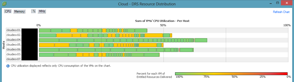
Naturally, the easiest way to fix this is to add additional physical CPU’s into the fold. We accomplished this by upgrading all of our E5620 processors (4-core) in our ESXi hosts to E5645 processors (6-core) thereby adding 28 additional cores to the platform. However, this did not help with CPU READY times. vSphere DRS was still reporting trouble delivering CPU resources to VM’s:

DRS-before-dbpm

After many hours of troubleshooting, we were finally about to find a solution – disabling DBPM. One of the hosts consistently showed lower CPU ready times even though it had higher density. We were able to find that this node had a different hardware power management policy than the other nodes. You can read more about what this setting does in the Host Power Management whitepaper from VMWare. By default, this policy is automatically set as a result of ACPI CPU C-States, Intel Speedstep and the hardware’s power management settings on the system.

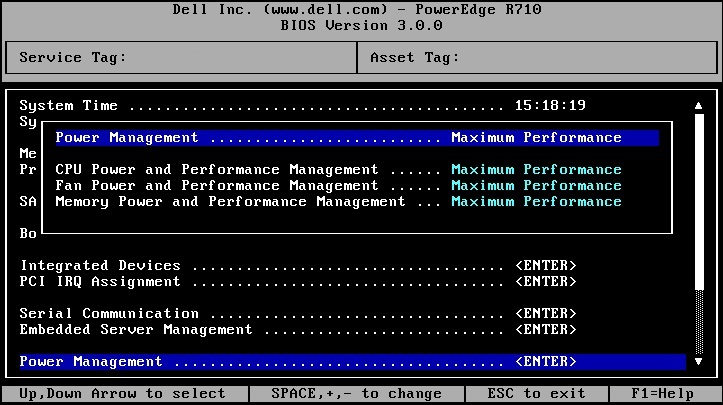
On our Dell Poweredge R610 host systems, the DBPM setting was under Power Management in the BIOS. Once we changed all systems from Active Power Controller to Maximum Performance, CPU ready times dropped to normal levels.

dell-r610-bios-power-management-settings

Information on the various options can be found in this Power and Cooling wiki from Dell. Before settling on this solution, we attempted disabling C-States altogether and C1E specifically in the BIOS, but neither had an impact. We found that we could also specify OS Control for this setting to allow vSphere to set the policy, though we ultimately decided that Maximum Performance was the best setting for our environment. Note that this isn’t specific to vSphere – the power management setting applies equally to all virtualization platforms.

Calculating disk usage and capacity using Diskmon

While evaluating SAN storage solutions for our VMWare environment, we found ourselves asking the question “How many systems can we fit on this system before IOPs and/or throughput become a bottleneck?” Come to find out, the answer is not a simple one. In fact, all of the vendors we posed this question to were only able to give us vauge performance numbers based on perfect conditions. We set out on a quest to quantify the capacity of each of the backend storage systems we tested.

Generally speaking IOPs is inversely proportional to the request size while throughput is proportional. This means that as the request size descreases the total number of IOPs increases while throughput decreases and vice versa. So when you see performance numbers that claim very high IOPs those are based on small requests and therefore throughput will be very minimal. In additional, disk latency and rotational speed can play a role in skewing these numbers as well. Sequential operations will produce much higher numbers than random operations. When we add RAID to the equation, we will see a difference in numbers depending upon whether the operation is a read or a write.

What does all this mean? It means that the performance capacity of a disk or storage device is determined by 3 main factors: Request Size, Random/Sequential operation, and Read/Write operation. There are other factors that can play a role, but focusing on these three factores will provide an estimation of the capacity of a disk, array or storage system. There are differing opinions as to what these numbers are in “real life.” The generally accepted view is that the average request size is 32K, 60% of transactions are random while 40% are sequential, and 65% are reads while 35% are writes. However, these numbers differ depending upon the application. The best way to determine these numbers for your environment is to capture statistics from production systems and average them together.

Fortunately, there is a nice utility for Windows that will allow you to get this information. The Diskmon utility: http://technet.microsoft.com/en-us/sysinternals/bb896646.aspx available from SysInternals (now part of Microsoft), will log every disk transaction with the necessary information.

Diskmon from SysInternals (now Microsoft)

Diskmon will begin capturing data immediately. To stop Diskmon from capturing data, click the magnifying glass in the toolbar:

Stop capture

You can then save the output to a text file by clicking the save button. I recommend capturing data during normal usage over a reasonable period of time. Also, it is best to minimize the Diskmon window to keep CPU usage to a minimum. The next step is to import the text file into Excel. I have provided a sample excel spreadsheet you can use as a template to perform the necessary calculations: server_diskmon.

Diskmon output to Excel spreadsheet

By taking a sampling from various systems on our network and using a weighted average, we calculated average of usage on our systems. In our case, we were using a common storage backend, and we wanted to categorize different systems into low (L), medium (M), and high (H) usage systems. We then assigned a percentage to each. By doing this, we can calculate the disk usage on the system if x% are low usage, y% medium usage, and z% high usage.

Weighted average of several systems on our network

We now have an accurate estimation of the Read Request Size, Random/Sequential percentages, and Read/Write percentages. If we feed these numbers into IOMeter, we can get a baseline of what the backend storage system can support. Divide that by our weighted average and we can find exactly how many systems our backend can support. If we look at point in time numbers, we can figure out the percentage of disk capacity being used:

Capacity of storage backend

I have put together a sample IOMeter configuration file containing the “real life” specification of 32K requests, 60% Random / 40% Sequential, and 65% Reads / 35% Writes.

Also, there’s a great comparison of SAN backends for VMWare environments here: http://communities.vmware.com/message/584154. Users have run the same real life test against their backend storage systems which will allow you to compare your devices performance with other vendors.

One side note when using IOMeter, be sure to set your disk size to something greater than the amount of cache in your backend storage systems in order to calculate raw disk performance. The configuration file I have provided uses a 8GB test file which should suffice for most installations.

Perfomance Monitor Perfomance Objects displays numbers only

There are a number of posts regarding a hotfix available for Windows 2000 to fix an issue where Performance Monitor displays only numbers for performance objects and counters. However, I came across this problem the other day on a Windows 2003 server. After searching for a while, I found a solution that worked: http://support.microsoft.com/?kbid=300956. Simply running the following command from the command prompt, restored the text values to the Performace Objects:

lodctr /R

Microsoft Update causes 100% CPU for svchost.exe process

<UPDATE>John Bigg brought to my attention a hotfix Microsoft recently released for Windows Installer 3.1 v2: http://support.microsoft.com/kb/916089 that fixes this specific issue. Thanks John!</UPDATE>

You may have noticed since switching to Microsoft Update to get your updates, that your computer is unresponsive after startup when you have Automatic Updates enabled. You’ll also experience this problem when connecting to the Microsoft Update site. Task Manager will show near 100% CPU usage and extremely high Disk I/O for the svhost.exe process. Running tasklist /SVC from the command line will show that the matching PID contains the wuauserv service. The only known current solution, is to revert back to Windows Update. The problem manifests itself in the fact that Microsoft Update will search all cached installs on your local PC; a very CPU and Disk intensive process.

To revert back to the standard Windows Update, connect to the Microsoft Update site. On the left pane, click “Change Settings”. In the next window, scroll down to the “To stop using Microsoft Update” section and select the “Disable Microsoft Update software and let me use Windows Update only” checkbox. Click “Apply Changes”.